PARTIAL ANSWERS
CS3343, Spring 2012, Final Exam, 7 Apr 2012

Directions: Do not spend too much time on any one problem. Try to give as short an answer as you can that still fully answers the question.


  1. (15) Hashing:
    1. Show the result of inserting the following strings into a hash table using the given hash function values shown. They should be inserted in the order given, using open addressing to resolve collisions, and proceeding to the next lower address on each collision: hash(ralph)=8, hash(henry)=10, hash(wayne)=8, hash(roger)=10, hash(hamish)=9, hash(hortense)=7.

      IndexKeyHash addr
      4
      5hortense7
      6hamish9
      7wayne8
      8ralph8
      9roger10
      10henry10
      11

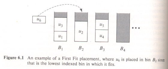
      [I gave credit to those who moved to higher addresses instead of lower ones. The question and its later parts still work in this case.]

    2. What would happen if we deleted the entry for wayne? (That is, made it an empty entry, ready for a new insertion.) With "wayne" changed to an empty entry, the look up of "hamish" and "hortense" would fail (saying that these are not present when they are).

      It is possible to have a special "deleted" type that functions as an full entry for look up, and in that case, the above searches would not fail.

    3. What is wrong with the following hash function, used for a hash table of size 50, where the keys are character strings. (The s.charAt(0) will use the Ascii code for the 0th character, so there's nothing wrong with that.) The worst thing about it is that it depends only on the first and last character of the string. In addition to summing all the characters, it would be better to also use the parameter p as a multiplier.

      int m = 50; // size of hash table
      
      public int hash(String s, int p, int m) {
         return (s.charAt(0) + s.charAt(s.length()-1))%m;
      }


  2. Quicksort and Randomization:
    1. Give the algorithm that randomizes the order of the elements in an array. What is it's asymptotic (time) performance? This elegant algorithm is half-way through the material on the page Randomize an Array.
    2. What is the worst-case asymptotic (time) performance of quicksort? O(n2)
    3. Explain how you could use Part i above to improve the performance of quicksort. Randomize the array to be sorted using part i before invoking quicksort. What kind of time performance does this give? Average-case time performance of O(n*log(n)). The worst-case performance is still O(n2) What "awkward" input case(s) does this help with? For your text's initial quicksort algorithm, one example is an array already in sorted order. Reverse sorted order is another example. Does this step eliminate these cases altogether? No, because for example, it is possible that the randomization would yield sorted order. If not, then why and how does this step help? For large n this is of vanishing small probability.
    4. Explain how the same technique would eliminate some of the same "awkward" input cases if one used a binary search tree for sorting. Randomizing the order before inserting into a binary search tree yields on average a depth (or height) bounded by 2*n*log(n). Searching would be efficient in such a tree: O(n*log(n)). Also: how would you use a binary search tree for sorting? Insert the array to be sorted into the binary search tree. Then output with an inorder traversal. What kind of performance does this "tree sort" algorithm have?
    5. Your text's Randomized Quicksort is different from Parts i and iii above. Explain the additions to the quicksort algorithm that give Randomized Quicksort. In the step of quicksort that partitions from index p to index r, generate a random integer i from p to r inclusive. Exchange the pivot in position A[r] with the element in A[i]. Then do the regular partition.


  3. (10) Adjacency List: Show the internal adjacency list representation of the graph in problem 4 below. Not much to this problem.


  4. (25) Breadth-First and Depth-First Searches of Graphs: By hand as we did in Recitation 13, run through a BFS and a DFS for the graph below, starting with vertex a. Assume that vertices are ordered alphabetically in the adjacency lists. Show the vertices in the order that they are visited. For each search you must use a stack or a queue, whichever is appropriate. Show the insertions and removals for each case. In each case the sequence of removals should be your final answer.

    [It was not necessary to fill out the full tables below, especially if the answer was correct.]

    Queue: add at right, remove from left
    BFS QueueActionAdd to Queue
    Initial -- Add a
    aRemove a and visit a  Add b, f 
    b fRemove b and visit bAdd c, d
    f c dRemove f and visit fAdd g
    c d gRemove c and visit cAdd e
    d g eRemove d and visit dAdd h
    g e hRemove g and visit gAdd -
    e hRemove e and visit eAdd -
    hRemove h and visit hAdd -
    BFS Order: a b f c d g e h
       
    Stack: push at right, remove from right
    DFS StackActionPush on Stack
    Initial -- Push a
    aPop a and visit a  Push b, f 
    b fPop f and visit fPush g
    b gPop g and visit gPush h
    b hPop h and visit hPush -
    b Pop b and visit bPush c, d
    c dPop d and visit dPush e
    c ePop e and visit ePush -
    c Pop c and visit cPush -
    DFS Order: a f g h b d e c


  5. (25) Dijkstra's Algorithm: By hand, run through Dijkstra's algorithm on the graph below, starting with vertex a. You should fill in the squares in the table below the graph, giving your answer. (You can also give your answer in another way, without the table, but you must be sure to show intermediate steps, especially the relax steps.) Below, a star (*) marks those vertices that have been removed from the priority queue and processed (visited). In this case it is not sufficient to give just the answer, since the directions ask for "intermediate steps".

     
    Action Contents of Priority Queue (* = removed)
    Remove
    & Relax
    abc d ef
    Initial0
    a0 *5 8
    b0 *5 *15 79
    d0 *5 *15 7 *9
    e0 *5 *10 7 *9 *14
    c0 *5 *10 * 7 *9 *12
    f0 *5 *10 * 7 *9 *12 *


  6. (20) Problems in NP: Note: this question has nothing to do with NP-completeness.
    1. Is any problem in P (polynomial-time problems) also in NP? Yes. Using the "guessing-stage / checking-stage" definition of NP below, we see that a problem in P satisfies this definition without making use of the guessing-stage at all.
    2. Is P the same as NP? Can you prove this? Most researchers think now that P is a proper subset of NP, but no one has been able to prove this.
    3. Give the "guessing-stage / checking-stage" definition that shows a problem is in NP. NP is the class of problems solvable on a nondeterministic computer. A nondeterministic computer can carry out a nondeterministic algorithm. Such an algorithm proceeds in two stages:
      1. Guessing stage: the algorithm "guesses" a structure S, which either is the answer to the problem or will help compute the answer.
      2. Checking stage: the computer proceeds in a normal deterministic fashion to use S in arriving at a Yes-No answer to the problem. The checking stage must be done in polynomial time. In effect S is the answer and the checking stage verifies in polynomial time that S is the answer.
    4. How would you use the definition in (iii) above to show that the problem Subset Sum (SS) is in NP? Here you start with a set A of positive integers and a given sum S. The problem is whether or not A has a subset A' whose numbers add up to S. During the guessing-stage, the algorithm guesses the correct answer A'. In the checking-stage the algorithm computes the sum of the numbers in A' and checks if this sum equals S.


  7. (20) Turing Machine: Consider the following "mystery" program in the language used for our Turing machines:

    Instructions in the Turing Language
    InstructionRepresentation Op
    Code
    print 0 000 0
    print 1 001 1
    move left 010 2
    move right 011 3
    stop 100 4
    if 0 is scanned
     goto i
    101 0...0 1
        <-i->
    5
    if 1 is scanned
     goto j
    110 1...1 0
        <-j->
    6
    (end marker) 111 -
     
    Mystery Program ??
    InstructionRepresentation
     1. print 0
     2. move right
     3. if 1 is scanned goto 2
     4. print 1
     5. move left
     6. if 1 is scanned goto 5
     7. move left
     8. if 0 is scanned goto 7
     9. print 0
    10. move left
    11. if 1 is scanned goto 10
    12. print 1
    13. move right
    14. if 1 is scanned goto 13
    15. move right
    16. if 0 is scanned goto 15
    17. if 1 is scanned goto 1
    18. stop
        (end marker)
    
    Initial   ...0001100011000...
     tape:               |
    
    000
    011
    110 11 0
    001
    010
    110 11111 0
    010
    101 0000000 1
    000
    010
    110 1111111111 0
    001
    011
    110 1111111111111 0
    011
    101 000000000000000 1
    110 1 0
    100
    111
    

    1. Explain carefully what this mystery program does. What is its output and what actions does it go through to produce this output? (All tape squares outside those shown are zero.) [As before I had a lot of trouble writing any program at all that would do something non-trivial. Very hard to write a program that will stop.]
        Original tape looks like:
        L = left segment of 1's, M = middle segment of 0's, R = right segment of 1's
        All 0's outside these segments, indefinitely far.
              <--L--><--M--><--R-->
        ...00011...1100...0011...1100...
        
        OK, here is what the program is doing:
        1.     Print 0 at left end of R.
        2-3.   Scan right to 1 past right end of R.
        4.     Print 1 at 1 past right end of R.
        5-6.   Scan left to 1 past left end of R (= right end of M).
        7-8.   Scan left to 1 past left end of M (= right end of L).
        9.     Print 0 at right end of L.
        10-11. Scan left to 1 past left end of L.
        12.    Print 1 at 1 past left end of L.
        13-14. Scan right to 1 past right end of L (= left end of M).
        15-16. Scan right to 1 past right end of M (= left end of R).
        17.    Now scanning the 1 at left end of R (same position relative to L, M, and R as at start).
               Will always goto step 1.  Start over.
        
        Effect of 1 time through loop: R and L stay the same length, and all of R moves right one square, and all of L moves left one square, and M has an extra 2 0's.
        As it runs, L and R pushed apart. Each loop, M has extra 2 0's.
      Here is simulation run of first 100 steps.

    2. Suppose the starting tape configuration were the following:

      Initial   ...00011100111000...
       tape:               |
      

      With this program, L, M, and R can be any length greater than or equal to 1, independent of one another. As the program runs, L and R will stay the same length and be pushed apart 2 squares during each loop. Here is simulation run of first 100 steps.


  8. (20) Example of Polynomial Time Equivalence. Consider the two problems:

    Consider also the two reductions L1 ≤p L2 and L2 ≤p L1.

    L1 ≤p L2 means to reduce the problem of solving L1 to the problem of solving L2. This means that we start with an instance of L1 and try to find a corresponding instance of L2 is such a way that the solution to the L2 instance gives us the solution to the L1 instance.

    Another way to say this is that assuming we can solve problems in L2, does that let us solve problems in L1?

    1. One of these reductions is trivial. Which one is "trivial" and why do I use that word.? The direction L1 ≤p L2 is the trivial one, because if we can take the square root of any positive number, we can certainly take the square root of any number in the range 1/4 <= x <= 1. Another way to say this is: given any desired sqrt(x) in the range 1/4 <= x <= 1, we associate it with exactly the same problem in the greater range, x > 0. If we can find sqrt(x) for any x > 0, then certainly we can find sqrt(x) for any 1/4 <= x <= 1.

    2. The other is something that we proved. What rough technique did we use to prove it? To prove the other direction: L2 ≤p L1, we start knowing that we can find sqrt(x) in the range 1/4 <= x <= 1. We start with an arbitrary sqrt(x), where x > 0. In this case we normalized the arbitrary case by multiplying or dividing repeately by 4, until our arbitrary problem was in the range 1/4 <= x <= 1. Then take the square root. Finally by dividing or multiplying by 2 to the same power as for normalization, we denormalize and get a solution to original square root.


  9. (20) Hamiltonian Cycles and Paths: Recall that a Hamiltonian Cycle (HC) is a path in an undirected graph that includes all vertices exactly once, and starts and ends at the same vertex. A Hamiltonian Path (HP) is a path that also includes all vertices exactly once, but it starts and ends at distinct vertices. (In this notation, an HC is not an HP, because an HC does not start and top at distinct vertices.)

    1. Did the undirected graph of the 48 states have a Hamiltonian Cycle? This graph cannot have a Hamiltonian cycle. In fact, the vertex 41 or NY is what's defined as an articulation point for this graph: "A vertex in a connected undirected graph is an articulation point if removing it and all edges incident to it results in a non-connected graph [Wikipedia]". In other words, such a vertex is a bottleneck through which all paths from one side to the other much travel. No graph with an articulation point can have a Hamiltonian cycle. Articulation points are important in many applications, such as in networks, where bottlenecks are important.

      Did it have a Hamiltonian Path? The problem of checking whether or not a given graph has a Hamiltonian path is NP-complete. We have displayed several Hamiltonian paths for this graph. Every such path much go through the vertex 41 as above. There are 68656026 distinct Hamiltonian paths in this graph.

    2. If you had a Hamiltonian Cycle in a Graph, explain how you could get a Hamiltonian Path. If you have a Hamiltonian cycle, just delete any single edge to get a Hamiltonian path. [More commonly, Hamiltonian paths are defined to include all Hamiltonian cycles (if any) as special cases.]

    3. Does a complete graph always have a Hamiltonian Cycle? A complete graph is undirected and has an edge between every pair of vertices. So you can arrange the vertices in any order (no repetitions) and put the first one on at the end; then you have a Hamiltonian Cycle.

    4. Let TS stand for the Traveling Salesman Problem. We proved something involving HC and TS. What was it? We proved that HC ≤p TS. To do this, we started with an instance of HC, and constructed a fairly simple instance of TS: Same vertices as the HC instance. Made a complete graph, with all edges that were in the HC instance having cost 1 and all other edges with cost 2. The bound on the cost was taken to be the number of vertices. Because of this, those vertices with cost 2 have to be ignored in a Hamiltonian circuit. See HC Reduces to TS for more details.

      At this point in your text's presentation, they had already proved that HC is NP-complete. This proof that HC ≤p TS, along with a proof that TS is in NP, is a proof that TS is also NP-complete.


  10. (20) Bin Packing: The Bin Packing Problem (BP) starts with a set of n objects, where the size si of the ith object satisfies 0 < si < 1. We also start with a number K of unit-size bins. The decision problem asks (with a "yes" or "no" answer) if we can pack all n objects into K bins. The BP decision problem is NP-complete. (We visualize that objects and bins all have base a unit square, and so all that matters is the height. For example, we can fit 8 objects of size 0.25 into 2 bins, by piling 4 into each bin.)

    1. State an optimization problem that corresponds to the decision problem above. You see, the decision problem is just: "Yes we can fit the objects into K bins", or "No, we can't". The optimiztion problem asks: "What is the minimum number of bins into which we can fit all the objects?"

    2. If we could solve the BP decision problem in time O(P(n)) for some polynomial p in the variable n, explain how we could solve the optimization problem in time O(P(n)*log(M)), where M is a number of bins that easily accommodates all the objects. Start with a specific instance of BP with bound K, call it, say (bp, bound K). Pick a bound M large enough so that (bp, bound M) = "yes". (For example, we could use M = number of objects.) If (bp, bound 0) = "yes" we are done. (This might be a problem with all sizes 0.) Now this proceeds in a way similar to binary search:
        We have the optimal value trapped between bounds L < R,
        where initially L = 0 and R = M.  Set Mid = (L + R)/2.
        
             L ("no")      Mid (?)       R("yes")
             |--------------|------------|
        
        if the bound of Mid gives a "yes" then change to:
             L ("no")       R ("yes)   
             |--------------|------------|
        
        and if bound of Mid gives a "no" then change to:
                           L ("no")     R ("yes)   
             |--------------|------------|
        
        In this way the optimal value is trapped between bounds
        whose distance apart in halved at each stage.  So in
        log2(M) steps, we will have the optimal value.
        

    3. There are several algorithms with give an approximate answer to bin packing, though not the exact optimal answer. One of these algorithms is called First Fit (FF). It assumes that we have an infinite sequence B1,B2,B3,... of unit-capacity bins. The algorithm places objects int the bins, processing objects in the order s1,s2,s3,... and placing each object into the bin with lowest index into which it will fit. Here's an illustration of this (where in this picture sizes are denoted by ui):

      Denote by OPT(P) the optimal number of bins needed for a BP problem P. Then let FF(P) be the number of bins required by FF. You should show that FF(P) requires at most 2*OPT(P)+1 bins. [Hint: every bin except one must be more than half full. Try to draw a picture in which several bins are half full or less.] [This is hard stuff!] Any 2 bins that are half full or less can be consolidated into 1 bin. Consider a first fit packing of objects into bins. All but one of these bins must be greater than half full, because otherwise we could consolidate bins. This means that

        FF(P) < 2 * sum(si: all i) + 1

      But all the object must fit into OPT(P) many bins.

        sum( si: all i) <= OPT(P)

      Combining inequalities gives:

        FF(P) < 2 * sum(si: all i) + 1 <= 2 * OPT(P) + 1

      In fact, it is possible to prove the bound:

        FF(P) < (17/10) * (sum(si: all i) - 1)

      There is an approximation algorithm First Fit Decreasing (FFD) that handles the objects in decreasing order of size. Anyone who had packed up a truck for moving knows that this is likely to give better results, and it does. In this case one can prove a bound:

        FFD(P) < (11/9) * sum(si: all i) + 4

      The two bounds above are quite difficult to prove (the proofs are not even presented in the advanced text I was using.) Bin Packing is only briefly discussed in your text, page 1134.