 |
| Textbook. |
Analysis of Algorithms
Fall 2012
Recitation 13
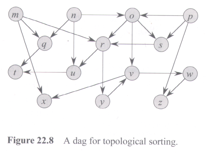
DFS, Etc.
Partial Answers
|
CS 3343 Analysis of Algorithms Fall 2012 Recitation 13 DFS, Etc. Partial Answers |
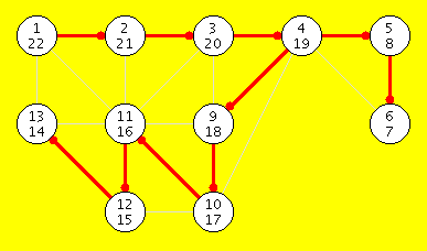
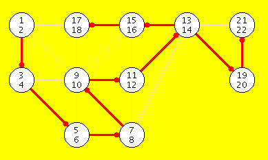
| Using Recursion, Start = 0 | Using a Stack, Start = 0 |
|---|---|
 |
 |
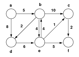
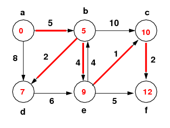
| Action | Contents of Priority Queue (* = removed) | ||||||
|---|---|---|---|---|---|---|---|
| Remove & Relax |
a, π | b, π | c, π | d, π | e, π | f, π | |
| Initial | 0, nil | ∞, nil | ∞, nil | ∞, nil | ∞, nil | ∞, nil | |
| a | 0, nil * | 5, a | ∞, nil | 8, a | ∞, nil | ∞, nil | |
| b | 0, nil * | 5, a * | 15, b | 7, b | 9, b | ∞, nil | |
| d | 0, nil * | 5, a * | 15, b | 7, b * | 9, b | ∞, nil | |
| e | 0, nil * | 5, a * | 10, e | 7, b * | 9, b * | 14, e | |
| c | 0, nil * | 5, a * | 10, e * | 7, b * | 9, b * | 12, c | |
| f | 0, nil * | 5, a * | 10, e * | 7, b * | 9, b * | 12, c * | |