This discussion uses the book's terminology on pages 170 and beyond. The quicksort algorithm uses a special function Partition to work on the portion of an array A[p .. r] where indexes p and r are in range with p < r. Partition finds an index q with p <= q <= r and rearranges A[p .. r] so that the subarray (which might be empty) A[p .. q-1] has each element <= A[q] and the subarray (which also might be empty) A[q+1 .. r] has each element >= A[q]. The array element A[q] is called the pivot.

At this point the algorithm Quicksort can call Partition recursively on the two subarrays (assuming they have more than one element):

Quicksort(A, p, r)
if p < r
   q = Partition(A, p, r)
   Quicksort(A, p, q-1)
   Quicksort(A, q+1, r)


The initial call is:

Quicksort(A, 1, A.length)

The above initial call is in the book's world. In our Java world the call would be Quicksort(A, 0, A.length - 1), and similarly for C.

Thus the only hard part is the partitioning function. There are many different partitioning functions, but your book has a somewhat exotic version. As part of the explanation, I'm going to illustrate how a normal partition works below, and then we can look at the book's version.

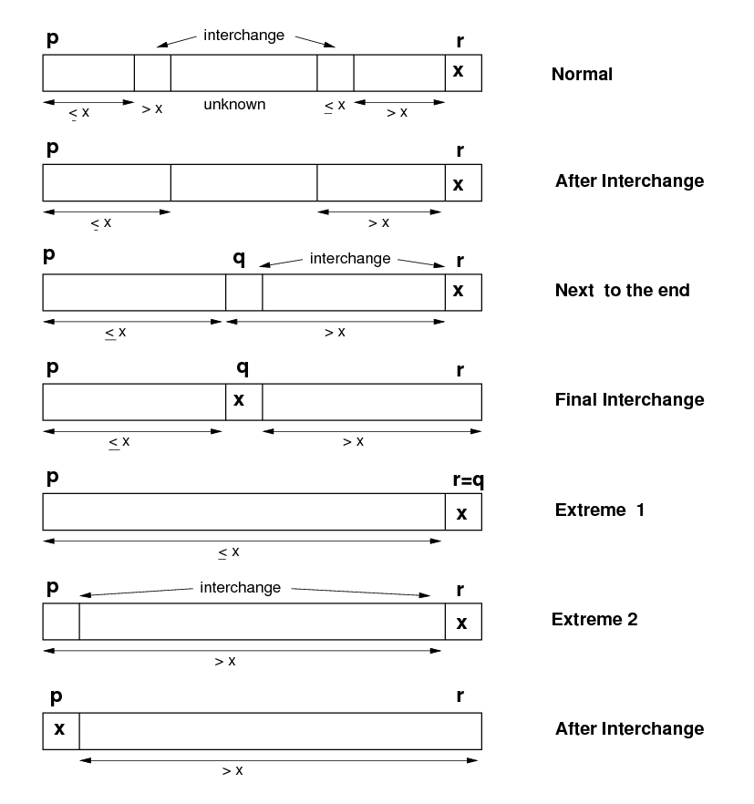
Both the book and the standard version below choose the element A[r] as the pivot, which they call x. Below it is at the right hand end of the array. The version below works toward the right from p and toward the left from r-1, looking toward the right for an element > x and toward the left for an element <= x. When (or if) two elements like these are found, then the algorithm interchanges them (see the top two diagrams below, labeled "Normal" and "After interchange".)

This process continues until we get to the state in the third diagram below. Then the elements in positions q and r are interchanged to give the fourth diagram. The fifth diagram gives an extreme possibility, where the pivot is >= all elements. In the sixth diagram, the pivot is < all elements, so it has to be interchanged with the initial element.

Full-size image: .png, .ps, .pdf.

The book's partition does pretty much the same as the above, except that the indexes and interchanges are arranged so that the "unknown" group of array elements is kept to the right of the others (but with the pivot x still to the right of everything.

Partition(A, p, r)
x = A[r]  // pivot
i = p - 1  // nothing small so far
for j = p to r - 1  // handle each elt in turn
   if A[j] <= x  // found one for small side
      i = i + 1  // find a place for it
      exchange(A[i], A[j]) // put small one in
exchange(A[i+1], A[r]) // move pivot to middle
return i + 1  // return pivot location

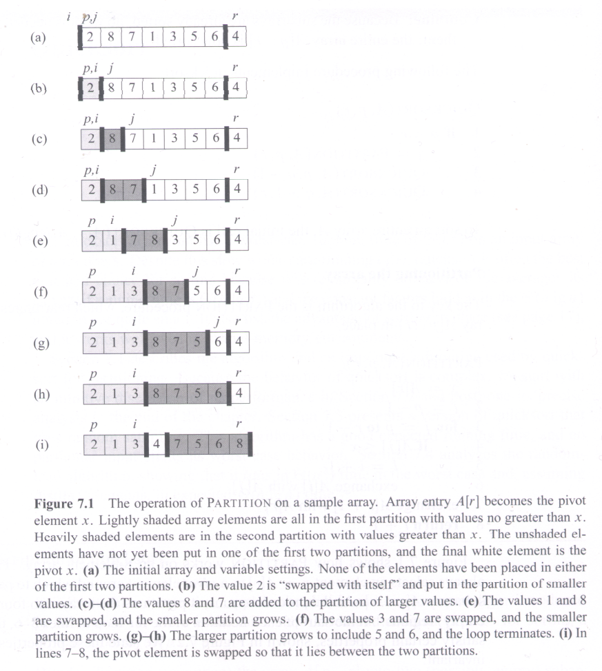
Here is your text's example of partitioning an array of 8 elements.

Full-size image: .png, .gif, .jpg.