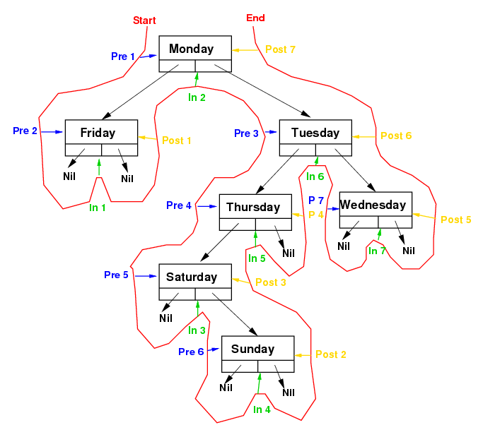
 Complete Tree Traversal (click picture or days.pdf). |
|
|
CS 3343/3341 Analysis of Algorithms |
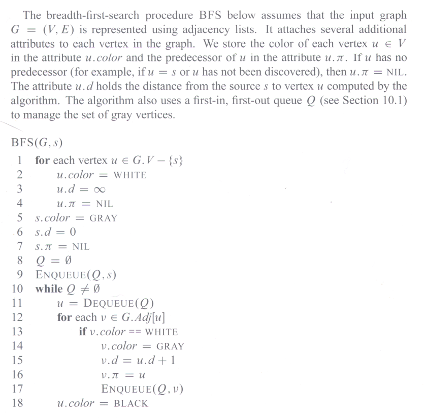
Graph Search
Breadth- and Depth-First |
|
Complete Tree Traversal (click picture or days.pdf). |
|
|
| Print-Path(s, v) if v == s print s elseif v.π == NIL print "no path from" s "to" v else Print-Path(s, v.π) print v |